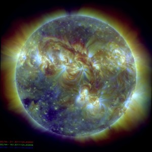
Thought I would share this video that was shared by NASAs SDO facebook page, I think it gives alot of background into the importance of solar research as well as it has some great info, visuals and history about solar weather.
Enjoy!
Tags: media
In a meeting with my advisers, it was said by one of their colleagues that the AIA 211 images might be more detailed in the features to detect. Since originally I decided to use AIA 193, because visually it was easier for me to see and identify the solar cavities, I decided to try the composite image of AIA 193, AIA 211 and AIA 171. I trained this new classifier with same dates as the AIA 193 classifiers in previous posts, but with the composite images of the same date. In testing the new classifier produced, I ran it initially against the training set that was used to create the classifier, as seen in the previous post. So now we are going to start running tests on new image sets, to see how it truly performs on images it has never “seen” before.
The below hit rate was achieved when running the new composite classifier against the above single image rotated by one degree for 360 degrees.
Hit rate ≈ 100%
You can see the hit rate achieved was greater than that on just the AIA 193 classifier, but the false alarm rate is also higher.
+================================+======+======+======+
|            File Name           | Hits |Missed| False|
+================================+======+======+======+
|20111124_002649_1024_211193171.j|     1|     0|    38|
+--------------------------------+------+------+------+
|1-DEG-24_002649_1024_211193171.j|     1|     0|    36|
+--------------------------------+------+------+------+
[...]
+--------------------------------+------+------+------+
|358-DEG-24_002649_1024_211193171|     1|     0|    35|
+--------------------------------+------+------+------+
|359-DEG-24_002649_1024_211193171|     1|     0|    40|
+--------------------------------+------+------+------+
|                           Total|   360|     0| 14157|
+================================+======+======+======+
Tags: haar training, performance, testing outcomes, trials
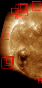
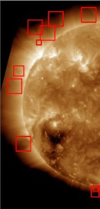
Now that a decent Hit Rate has been achieved, the focus turns to reducing the False Alarms. One step to reducing the false alarms is to eliminate overlapping regions of interest, so that the false alarms picked up in about the same vicinity will count as 1 or 2 false alarms as opposed to 6 or 7.
Original False Alarm count was 95058, after some implementation on blocking out the suns disk the count drop to 79702.
This reduces the false alarms by 15356 which is about ≈ 16%.
Below is a coding excerpt for the function to eliminate regions of interest that overlap with other regions of interest. This is a very overly simple way of eliminating regions, this method could be extended to be more discriminating as well as smarter in its selection. The current method =, simply checks if the center point of a new region lies within the bounds of an already existing region.
//!**************************************************
//! @details
//! This function is to determine if our new region of interest
//! overlaps any previous regions of interest in this image
//!
//! @param [in] <CvRect region>
//! The new region of interest in the image
//!
//! @return <bool bRegionOverlaps>
//! Boolean for whether this region overlaps a previous region of interest
//!**************************************************
bool DoRegionsOverlap(CvRect region)
{
	bool bRegionOverlaps = false;
	vector<CvRect>::iterator it;
	for ( it = m_RegionsOfInterest.begin() ; it < m_RegionsOfInterest.end(); it++ )
	{
		//Is the center point contained in another region
		int centerx = region.x + (region.width / 2);
		int centery = region.y + (region.height / 2);

		if (centerx >= it->x && centerx <= (it->x + it->width))
		{
			if (centery >= it->y && centery <= (it->y + it->height))
			{
				//TODO: Only keep the region that has the biggest area
				bRegionOverlaps = true;
				break;
			}
		}
	}

	return bRegionOverlaps;
}
Tags: performance, testing outcomes, thesis, trials
Now that a decent Hit Rate has been achieved, the focus turns to reducing the False Alarms. One step to reducing the false alarms is to black out the suns disk, so that the false alarms picked up in the suns disk will eliminated from the count.
Original False Alarm count was 95058, after some implementation on blocking out the suns disk the count drop to 85725.
This reduces the false alarms by 9333 which is about ≈ 10%.
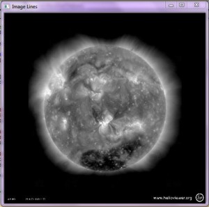
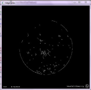
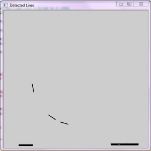
Below is a coding excerpt for the function to Black out the suns disk. First we blur the image slightly, followed by running the Canny edge detector on the image. Once the edges are found the HoughLines algorithm is run to find all the line segments in the image. Using these methods we are trying to determine a radius to the suns edge to then determine our circle size.
//!**************************************************
//! @details
//! This will first perform Canny detection on the image
//! once the edges are found it will find the lines of the edges
//! using the Hough transform. Which will get the radius of the area
//! to black out.
//!
//! @return <bool bProcessed>
//! Whether we were able to process any lines found.
//!**************************************************
bool BlackOutTheSun()
{
	Mat cdst;
	bool bProcessed = false;
	cdst.create(image.size(), image.type());
	blur(image, edge, Size(3,3));

	// Run the edge detector on grayscale
	Canny(edge, edge, edgeThresh, edgeThresh*3, 3);
	cedge = Scalar::all(0);

	image.copyTo(cedge, edge);

	vector<Vec4i> lines;
	HoughLinesP(cedge, lines, 1, CV_PI/180, 50, 50, 10 );
	float slope;
	for( size_t i = 0; i < lines.size(); i++ )
	{
		Vec4i l = lines[i];
		line( cdst, Point(l[0], l[1]), Point(l[2], l[3]), CVX_RED, 3, CV_AA);

		// Make sure we don't get into a divide by 0 state
		if((l[0] - l[2]) != 0)
		{
			slope = static_cast<float>((l[1] - l[3]) / (l[0] - l[2]));

			if(abs(slope) >= 1)
			{
				m_nfoundX = l[0];
				m_nfoundY = l[1];
			}
			bProcessed = true;
		}
	}
	cvNamedWindow("Edge Lines", CV_WINDOW_NORMAL);
	imshow("Edge Lines", edge);
	waitKey(0);

	cvNamedWindow("Image Lines", CV_WINDOW_NORMAL);
	imshow("Image Lines", image);
	waitKey(0);

	cvNamedWindow("Detected Lines", CV_WINDOW_NORMAL);
	imshow("Detected Lines", cdst);
	waitKey(0);

	return bProcessed;
}
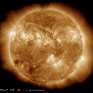
Below are examples of the image outputs from the operations in the above code excerpt.
Tags: performance, testing outcomes, thesis, trials
In testing the classifiers produced, I ran it initially against the training set that was used to create the classifier, as seen in the previous post. So now we are going to start running tests on new image sets, to see how it truly performs on images it has never “seen” before.
The below hit rate was achieved when running the new classifier against the above single image rotated by one degree for 360 degrees.
Hit rate ≈ 90%
+================================+======+======+======+
|            File Name           | Hits |Missed| False|
+================================+======+======+======+
|   20111124_002656_1024_0193.jpg|     1|     0|    21|
+--------------------------------+------+------+------+
|   1-DEG-24_002656_1024_0193.jpg|     1|     0|    28|
+--------------------------------+------+------+------+
[...]
+--------------------------------+------+------+------+
| 358-DEG-24_002656_1024_0193.jpg|     1|     0|    20|
+--------------------------------+------+------+------+
| 359-DEG-24_002656_1024_0193.jpg|     1|     0|    25|
+--------------------------------+------+------+------+
|                           Total|   324|    36| 10341|
+================================+======+======+======+
Tags: haar training, performance, testing outcomes, trials
Through this process I have been trying to increase my sample sets, so I am currently up to about 3600 positive images resulting from rotating one positive image and tracking the ROI (region of interest) across all subsequent images, as well as increasing the negative set. Below are the commands and parameters used to create this specific classifier as well as the outcomes and stats from the performance application.
CreateSamples
G:\CreateSamples\Debug>CreateSamples.exe -info "G:\Thesis Research\Test Sets\Positi

ves_With_Rotations\Markup_List.txt" -vec "G:\Thesis Research\Test Sets\Positive

s_With_Rotations\Markup_List_Zangle2_3000Samples.vec" -num 3000 -maxzangle 1.1
Training
OpenCV2.2\bin>opencv_haartraining.exe -data "C:\Thesis Research Runs\HaarClas

sifier\haarcascade_21" -vec "C:\Thesis Research Runs\Test Sets\Positives_With_Rot

ations\Markup_List_Zangle2_3000Samples.vec" -bg "C:\Thesis Research Runs\Test Se

ts\Negative Solar Cavities\extended_negatives_3342.txt" -npos 3600 -nneg 3342 -n

stages 20
Performance
C:\OpenCV2.2\bin>opencv_performance.exe -data "C:\Thesis Research Runs\HaarClass

ifier\haarcascade_21\haarcascade_21.xml" -info "C:\Thesis Research Runs\Test Sets\

Positives_With_Rotations\Markup_List.txt" -maxSizeDiff 2
So the below chart shows the distribution of HITS, MISSES and FALSE ALARMS. For this training set I used the default -maxfalsealarm setting to have the trainer finish quickly. The results reflect this by showing such a high false alarm rate. Which is fine right now, since I feel we are on a better path with trying to get the HIT count up. So then we can go about it the same way and let the trainer run for longer to reduce the false alarms as well as do some filtering implementations to alleviate ones that we know are not “true” cavities.
The below hit rate was achieved when running the new classifier against the initial training set.
Hit rate ≈ 95.5%
Tags: testing outcomes, trials
When creating samples from the marked images the default options are listed below. You notice that the default for the maxzangle is less than the defaults for the x and y angle values. So why is that? What do these parameters mean?
C:\OpenCV2.2\bin>opencv_createsamples.exe
Usage: opencv_createsamples.exe
  [-info <collection_file_name>]
  [-img <image_file_name>]
  [-vec <vec_file_name>]
  [-bg <background_file_name>]
  [-num <number_of_samples = 1000>]
  [-bgcolor <background_color = 0>]
  [-inv] [-randinv] [-bgthresh <background_color_threshold = 80>]
  [-maxidev <max_intensity_deviation = 40>]
  [-maxxangle <max_x_rotation_angle = 1.100000>]
  [-maxyangle <max_y_rotation_angle = 1.100000>]
  [-maxzangle <max_z_rotation_angle = 0.500000>]
  [-show [<scale = 4.000000>]]
  [-w <sample_width = 24>]
  [-h <sample_height = 24>]
The Haar Classifier was initially developed for facial detections, but has been proven to be a good detection method in detecting other objects, as long as you specify the parameters correctly and robustly enough to have a representative set.
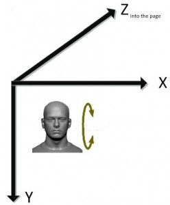
[-maxxangle <max_x_rotation_angle = 1.100000>]
So for the x angle value this correlates to rotations along the X axis, which in facial detection refers to looking up and down. So when you run create samples it will create samples based on this rotation specification to take that case into consideration in your training model.
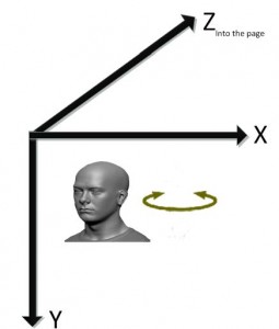
[-maxyangle <max_y_rotation_angle = 1.100000>]
For the y angle value this correlates to rotations along the Y axis, which in facial detection refers to looking left and right. So when you run create samples it will create samples based on this rotation specification to take that case into consideration in your training model.
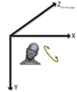
[-maxzangle <max_z_rotation_angle = 0.500000>]
For the z angle value this correlates to rotations along the Z axis, which is the axis that goes straight into the computer screen (image) and straight toward you. So in facial detection refers to tilting your head from side to side. So when you run create samples it will create samples based on this rotation specification to take that case into consideration in your training model.
If we think of our solar cavity circular form as the circular form of a face this correlates to x representing a cavity more upright and straight in orientation, y representing more of an oblong form transformed inward from the sides and z representing our cavities at an angle. So for solar cavities the majority of them seem to be at an angle as opposed to straight upward in orientation. For facial detection purposes the x and y make more sense as people rarely walk around, take pictures etc. with their heads tilted from side to side, but in relation to this research the z angle value is more important for our detection purposes, so we need to increase this value.
Tags: create samples, Haar Classifier, haar training, opencv, thesis
In the previous post Advanced Object Marker ::: [Tracking defined ROI (Region Of Interest)] the second video shows the new region of interest (ROI) as the YELLOW rotated rectangle. For our training purposes, a rotated rectangle can not be input to the training application as it expects the defining members of a rectangle as x, y, width and height. With x and y repseenting the upper left most corner of the box. To get around this we will simply create a bounding box for our rotated rectangle.
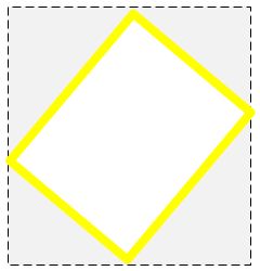
OpenCV has a built in class called RotatedRect for handling rotated rectangles as well as a helper function that will return the bounding rectangle (box) of the rotated rectangle. But for our purposes we do not want to rotate a rectangle by its center point but along the top left anchor point.
class RotatedRect
{
public:
    // constructors
    RotatedRect();
    RotatedRect(const Point2f& _center, const Size2f& _size, float _angle);
    RotatedRect(const CvBox2D& box);

    // returns minimal up-right rectangle that contains the rotated rectangle
    Rect boundingRect() const;
    // backward conversion to CvBox2D
    operator CvBox2D() const;

    // mass center of the rectangle
    Point2f center;
    // size
    Size2f size;
    // rotation angle in degrees
    float angle;
};
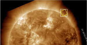
So because we know the endpoints that make up our rotated rectangle we can then form the bounding box for the region of interest (ROI). Below is a little code excerpt that uses the rotated rectangle positions to find the upper most x and y values as well as the lowest most x and y values of that rectangle. Once the loop is completed we know what our top left most point will be as well as our bottom right most point which we can then use to get our width values and height values to form the rectangle.
for (int i = 0; i < NUMBER_OF_PTS_ON_RECT; i++)
{
	//Find the lowest values
	if(lowestX > box_vtx[i].x)
	{
		lowestX = cvRound(box_vtx[i].x);
	}
	if(lowestY > box_vtx[i].y)
	{
		lowestY = cvRound(box_vtx[i].y);
	}

	//Find the greatest values
	if(greatestX < box_vtx[i].x)
	{
		greatestX = cvRound(box_vtx[i].x);
	}
	if(greatestY < box_vtx[i].y)
	{
		greatestY = cvRound(box_vtx[i].y);
	}

}
Tags: image processing, opencv
Now that we have eliminated scaling from our rotation images, we can now try to track/follow our region of interest (ROI) throughout all rotations. Below is the first initial attempt, we marked our first ROI so we know the left most point of the rectangle as well as its dimensions (width and height). So we then derived the new left most point of the shifted rectangle.
The GREEN box is the one that I initially marked, and the BLUE boxes are the ones that are derived from the original marked ROI and the shift in angle rotation. So it is supposed to track the ROI through all rotations. As you can see this is not handled quite right. The upper left hand corner of the box which is always the starting point of cvRect structure, does in fact follow the shift position at each rotation but the actual area of the rectangle is wrong. For example when we get to about degree rotation 90, the box should be inverted, as to cover the area but it still assumes a top down orientation from our rotation point.
In order to overcome this problem a rotation on the derived rectangle would be necessary. OpenCV does not draw rectangles at a rotation, so instead of needing just one point, width and height to describe an upright rectangle, we need to know all the points in the rotated rectangle.
//Get the distance from the center to our point of interest
int a = x - src_center.x;
int b = y - src_center.y;
double distance = sqrt((double)((a*a) + (b*b)));

//Convert the angle to radians
double radians = angle * (PI/180);

//Get the deltas (changes) in our x and y coordinate from our formula above
float deltaX = cos(radians) * a + sin(radians) * b;
float deltaY = cos(radians) * b - sin(radians) * a;

//Add the delta (change) values to our initial point value to get the shift and new coordinates
float newXPos = src_center.x + deltaX;
float newYPos = src_center.y + deltaY;

//Get the rotated rectangle values, from our ROI rotated at a angle value
cv::RotatedRect rect = RotatedRect(cvPoint((newXPos + (widthOfROI/2)), (newYPos + (heightOfROI/2))), Size2f(widthOfROI, heightOfROI), abs(angle));

//Create a holder for 4 points of our rotated rectangle.
CvPoint2D32f box_vtx[4];
cvBoxPoints(rect, box_vtx);
Once you have your 4 points in your rotated rectangle all you then need to do is loop through each point and draw a line connecting each one together, which results in a box drawn on your image. In the below video clip the GREEN box is our initial marked ROI, the BLUE box is our initial tracking implementation that assumed a top down orientation from the top left most corner point that we referenced and the YELLOW box is the new implementation that includes rotating the derived ROI (BLUE box) based on the anchored point in the upper left most corner, which you will notice the BLUE and YELLOW are always anchored at the same point in all rotations.
Tags: image processing, media, opencv, solar cavity
So initially we thought to rotate the image 1 degree and save the resulting image, we then ended up with about 360 image files derived from a single image. If we marked just the initial image (non-rotated) then based off of the placement in that image we could derive the position of interest in all subsequent images. With this technique there were a few problems encountered.
Below is an example of the images and their rotation. You will notice that along with the rotation there was also significant scaling to the image. So not only would we have to derive the position from the rotation but also the scaling.
So, I decided to simplify the situation and alleviate the scaling portion and only focus on the rotation. Below is a code excerpt that rotates an image about the center point and also keeps the original scale. Which is fortunate in our case that our images do not contain any useful information on the edges of the frame so if we lose the edges it does not hurt our purposes at all since its just black space.
//!****************************************************************
//! @details
//! This method rotates an image by a angle (degree) value
//!
//! @param [in,out] const Mat& source
//! The Mat image to rotate
//!
//! @param [in] double angle
//! The angle (degree) of rotation
//!
//! @return Mat dst
//! The resultant destination image after rotation
//!****************************************************************
Mat RotateImage(const Mat& source, double angle)
{
   //Get the center point of the image
	Point2f src_center(source.cols/2.0F, source.rows/2.0F);
	Mat rotation_matrix = getRotationMatrix2D(src_center, angle, 1.0);

//Show the rotation matrix
//cvNamedWindow( "Rotation Matrix", CV_WINDOW_NORMAL );
//imshow("Rotation Matrix", rotation_matrix);
//waitKey(0);
//cvDestroyWindow("Rotation Matrix");

	Mat dst;
	warpAffine(source, dst, rotation_matrix, source.size());
	return dst;
}
Below is an example of the images and their rotation. You will notice that along with the rotation there was no significant scaling to the image. So we no longer have to derive the position of the region based on the rotation and scaling.
Tags: image processing, media, opencv, solar cavity
